
Python GUIs
We’ve created an educational Graphical User Interface (GUI) in Python intended to teach students about MRI. The GUIs are very similar in design to the Tabletop GUIs, which are in MATLAB. The GUI is composed of a series of GUIs, each of which has its own function. These are:
- FID
- Spin Echo
- Signals
- 1D Projection
- 2D Imaging
- 3D Imaging
- Real-time Rotation
On this page, we provide a description of each GUI and how to use it.
Sockets
The Python GUI communicates with the server on the Red Pitaya via an abstraction known as a socket. A socket is an internal endpoint for sending or receiving data over a computer network. The client and server are both processes. In the client-server model, each process (i.e., the client and the server) establishes its own socket. The server socket resides at a particular IP address and, if used with TCP (as we do), requires a port number. The client socket needs to perform the following functions:
- Create a socket
- Connect the socket to the address of the server
- Send and receive data with the functions read() and write()
The server socket does the following:
- Create a socket
- Bind the socket to an address and port 3. Listen for a client on the port
- Accept a connection to a client
- Send and receive data
Our sockets use the reliable, stream-based TCP (Transmission Control Protocol) protocol to communicate over the network. On the client side, we used the software package PyQt’s QTCPSocket(), which provides useful abstractions. On the server side, we used the functions and abstractions defined in C’s native socket.h header file. In data transfer, the key functions were to read() and write() to the buffer.
Setup
In order to communicate with the Red Pitaya, you need to run the server program on it. First, ssh into the Red Pitaya. You need to have a static IP address set on it (follow the Red Pitaya documentation.
ssh root@[IP address]
Then, cat the bitfile:
cat pulsed_nmr_planB_05192018.bit >/dev/xdevcfg
Now run the server:
./server/mri_lab_rt 60 32200
(or whatever folder the server program is located in). The first argument, 60, is the length of the 90 degree hard RF pulse in samples. The second argument, 32200 is the amplitude of the pulse (arbitrary units). The program is mri_lab_rt.c in the server folder. We provide a pre-compiled binary, but you can also compile it yourself with the command:
arm-linux-gnueabihf-gcc -static -O3 -march=armv7-a -mcpu=cortex-a9 -mtune=cortex-a9 -mfpu=neon -mfloat-abi=hard /path/to/input.c -o output_file -lm
Once you have the server running, the GUI can connect to it. If using the anaconda environment, activate it:
Windows: activate ocra_env
macOS and Linux: source activate ocra_env
Now run the GUI script:
python runMRI.py
You should see the following page:
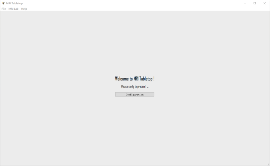
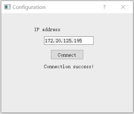
Make sure that you are running python3 (any version of 3 should work, 3.4 and 3.6 have been tested). In order to use any of the GUIs, you need to connect to the server by entering the IP address. Press the Configuration button, then enter the IP address of the Red Pitaya. If the connection is successful, you will see the following window:
FID GUI
In this GUI, you can acquire FIDs, find the center frequency, and adjust the B0 field via first-order shims. A labeled screenshot is shown below.
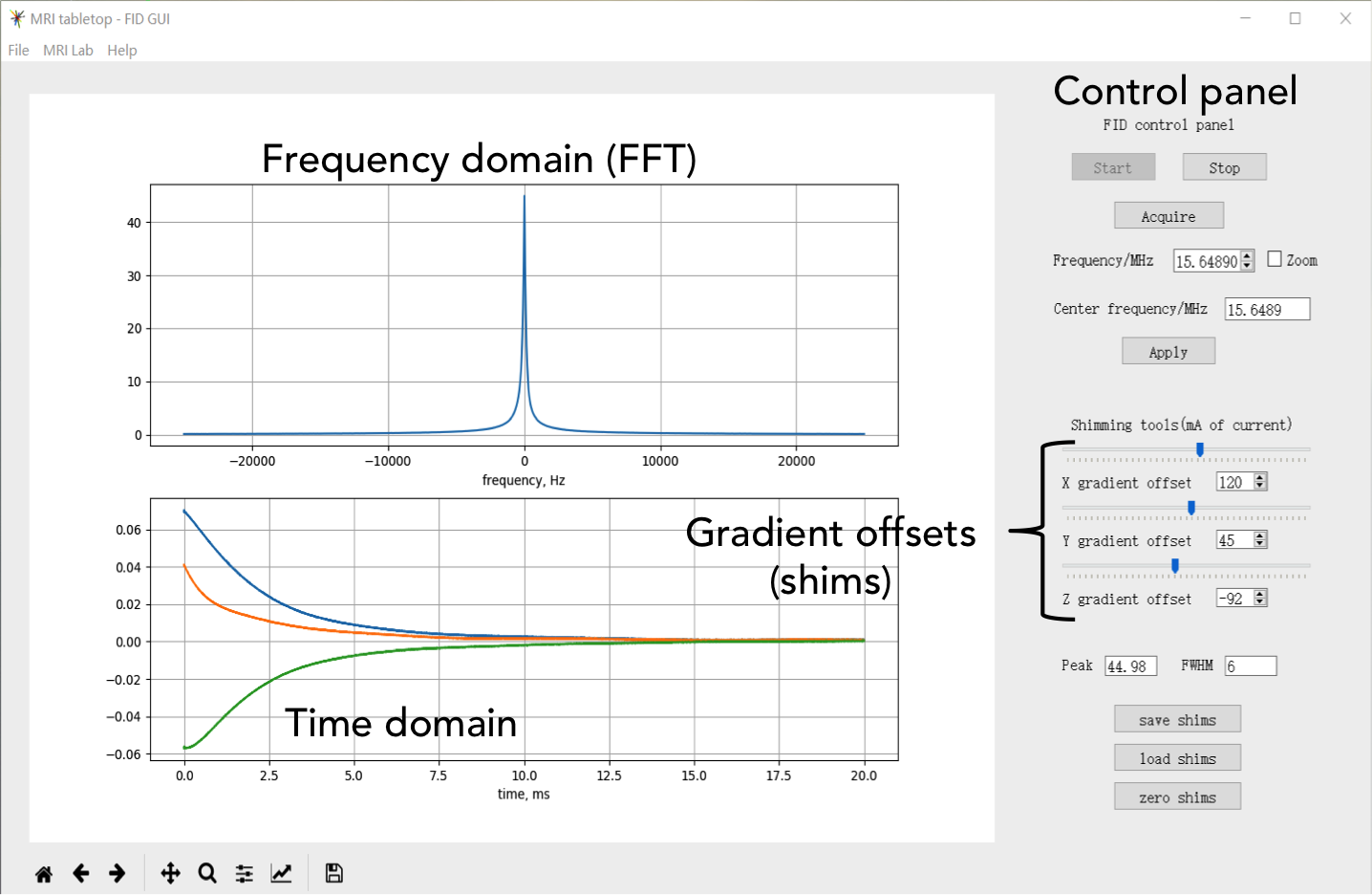
All GUIs share a time-domain plot, frequency domain plot, and control panel. In the control panel, you can start and stop the connection to the server with the “Start” and “Stop” buttons.
Press the “Acquire” button below the Start and Stop buttons to acquire data. You can adjust the center frequency manually, by pressing the arrows or entering a number in the text box, or automatically - the box below the manual adjustment finds the center frequency automatically. By pressing “Apply”, you can set the center frequency to the found peak.
Finally, the remainder of the control panel is devoted to shims. There are three first order shims in the Tabletop system: x, y, and z.
The values of the shims can be adjusted via the sliders or the arrows next to the text box. The GUI calculates the peak of the FFT magnitude and
FWHM to help determine the goodness of the shim. Once an optimal shim is found, you can save it by clicking on the “save shims” button,
where it will be saved for this session. The saved values will be automatically loaded in the other GUIs.
To have your saved shims appear on startup, modify the gradient_offsets attribute in the script basicpara.py. This is a list of three integers
for each shim in the format [shim_x, shim_y, shim_z]. You can also change the center frequency on startup by changing the freq attribute.
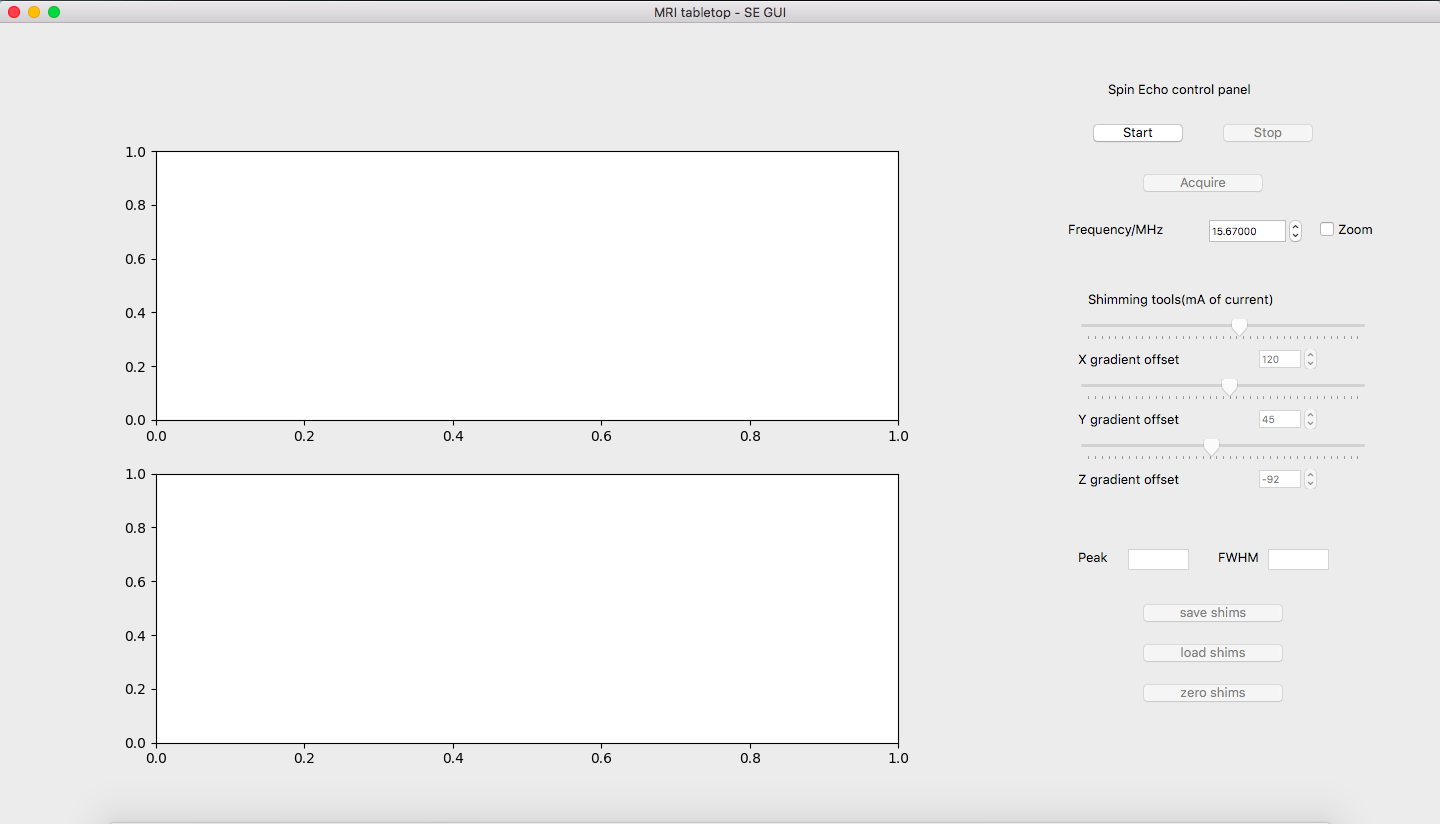
Spin Echo GUI
The Spin Echo GUI is very similar to the FID GUI, except that it acquires spin echoes instead of FIDs. A screenshot is shown below:
Signals GUI
The Signals GUI is an integrated GUI to test out sequences. Sequences are written in a custom Assembly-like language, which is described in the Sequence Programming section. Sequences are saved as .txt files and uploaded via the GUI. The GUI is pictured below.
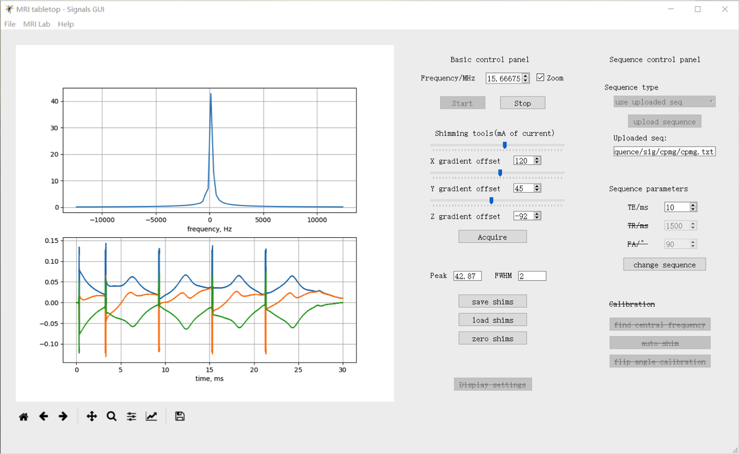
There are the same time domain plot, frequency domain plot, and shim control panel as in the FID and spin echo GUIs.
Additionally, there is a Sequence control panel. Here, you can upload sequences and adjust parameters (e.g. TE).
There are some example sequences provided in the sequence folder. Full descriptions of the sequences are in the
Sequence Programming section.
2D Imaging GUI
In this GUI, you can acquire 2D images, using one of our sequences or your own custom sequence. You can select the desired image size from a dropdown bar. The GUI updates the acquired kspace data and reconstructed image in real-time. A labeled screenshot is shown below.
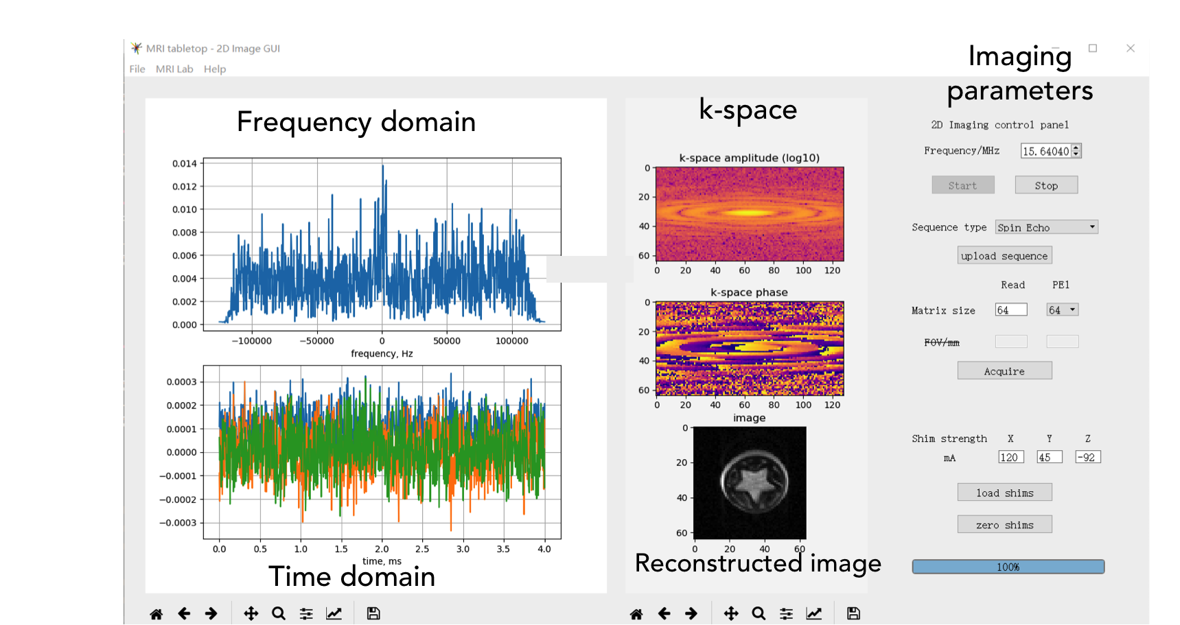
As in the other GUIs, press the “Start” button to start the connection to the server. Then, select a sequence type from the dropdown bar (e.g. “Spin Echo”, “Gradient Echo”) and upload a sequence. The provided sequences are .txt files in the sequence folder, described in the Sequence Programming section.
Then, select a matrix size. The image must be square and ranges from 4x4 to 256x256. Note that saving the data becomes much slower as the image size increases. Press the Acquire button to acquire the image. The kspace data and reconstructed image will refresh in real-time.
In this GUI, the shims are loaded from previous settings and cannot be modified. The center frequency can be adjusted.
3D Imaging GUI
In this GUI, you can acquire 3D images of a desired size. However, real-time reconstruction is not integrated and must be done outside of the GUI, e.g. via MATLAB. The GUI saves each partition as a different .mat file with the filename acq_data_N.mat, where N is the partition number. For instance, if there are 4 partitions, there will be 4 saved .mat files - acq_data_1.mat through acq_data_4.mat. You can change the filename via the fnameprefix attribute. A screenshot of the GUI is shown below.
<img src=https://openmri.github.io/ocra/assets/images/gui/3d_gui.png alt=”3d_gui” width=”700px”/>
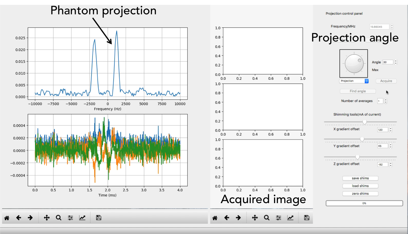
Real-time Rotation GUI
This GUI is a simple demonstration of motion correction for a phantom with two tubes of water. If the phantom is inserted at an arbitrary angle, the console will correct the orientation of the gradients such that the two tubes are horizontal in the image of the phantom. The GUI is pictured below.
The client (GUI) sends the current angle of the projection to the server, and the server rotates the gradients via multiplication with a rotation matrix. This is shown in the diagram below.
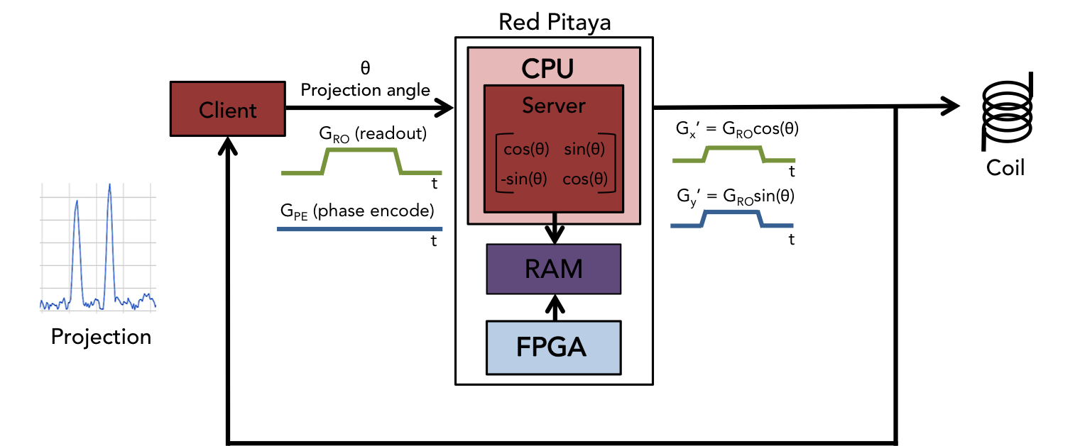
Then, the client performs a binary search to find the projection at which the two tubes collapse into one (the 0° projection in the diagram below):
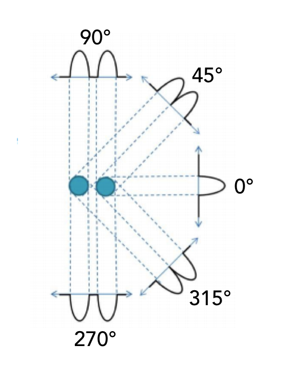
The binary search is as follows: if the current max is greater than the previous max, increase the angle. If the current max
is less than the previous max, decrease the angle and decrease the step size. If the step size is less than the tolerance, return
the max angle. The angle at which the two tubes are horizontal is 90° offset from the 0° angle.
To use the GUI, press Start. Select from the dropdown bar whether you want to acquire a 1D projection or a 2D image (spin echo, 64x64, TE=10ms). You can turn the dial to adjust the angle or use the arrowkeys. Press the “Find angle” button to perform the binary search and find the max angle. The value for the max angle will appear in the box next to the word “Max” once the search terminates.